The Blessing and the Curse of Dimensionality

A paper recently caught my eye, and I think it is a great excuse to talk about data scale and dimensionality.

Vatanen, T. et al. The human gut microbiome in early-onset type 1 diabetes from the TEDDY study. Nature 562, 589–594 (2018). (link)

In addition to having a great acronym for study of child development, they also sequenced 10,913 metagenomes from 783 children.

This is a ton of data.

If you haven’t worked with a “metagenome,” it’s usually about 10-20 million short words, each corresponding to 100-300 bases of a microbial genome. It’s a text file with some combination of ATCG written out over tens of millions of lines, with each line being a few hundred letters long. A single metagenome is big. It won’t open in Word. Now imagine you have 10,000 of them. Now imagine you have to make sense out of 10,000 of them.

Now, I’m being a bit extreme – there are some ways to deal with the data. However, I would argue that it’s this problem, how to deal with the data, that we could use some help with.

Taxonomic classification

The most effective way to deal with the data is to take each metagenome and figure out which organisms are present. This process is called “taxonomic classification” and it’s something that people have gotten pretty good at recently. You take all of those short ATCG words, you match them against all of the genomes you know about, and you use that information to make some educated about what collection of organisms are present. This is a biologically meaningful reduction in the data that results in hundreds or thousands of observations per sample. You can also validate these methods by processing “mock communities” and seeing if you get the right answer. I’m a fan.

With taxonomic classification you end up with thousands of observations (in this case organisms) across X samples. In the TEDDY study they had >10,000 samples, and so this dataset has a lot of statistical power (where you generally want more samples than observations).

Metabolic reconstruction

The other main way that people analyze metagenomes these days is by quantifying the abundance of each biochemical pathway present in the sample. I won’t talk about this here because my opinions are controversial and it’s best left for another post.

Gene-level analysis

I spend most of my time these days on “gene-level analysis.” This type of analysis tries to quantify every gene present in every genome in every sample. The motivation here is that sometimes genes move horizontally between species, and sometimes different strains within the same species will have different collections of genes. So, if you want to find something that you can’t find with taxonomic analysis, maybe gene-level analysis will pick it up. However, that’s an entirely different can of worms. Let’s open it up.

Every microbial genome contains roughly 1,000 genes. Every metagenome contains a few hundred genomes. So every metagenome contains hundreds of thousands of genes. When you look across a few hundred samples you might find a few million unique genes. When you look across 10,000 samples I can only guess that you’d find tens of millions of unique genes.

Now the dimensionality of the data is all lopsided. We have tens of millions of genes, which are observed across tens of thousands of samples. A biostatistician would tell us that this is seriously underpowered for making sense of the biology. Basically, this is an approach that just doesn’t work for studies with 10,000 samples, which I find to be pretty daunting.

Dealing with scale

The way that we find success in science is that we take information that a human cannot comprehend, and we transform it into something that a human can comprehend. We cannot look at a text file with ten million lines and understand anything about that sample, but we can transform it into a list of organisms with names that we can Google. I’m spending a lot of my time trying to do the same thing with gene-level metagenomic analysis, trying to transform it into something that a human can comprehend. This all falls into the category of “dimensionality reduction,” trying to reduce the number of observations per sample, while still retaining the biological information we care about. I’ll tell you that this problem is really hard and I’m not sure I have the single best true angle on it. I would absolutely love to have more eyes on the problem.

It increasingly seems like the world is driven by people who try to make sense of large amounts of data, and I would humbly ask for anyone who cares about this to try to think about metagenomic analysis. The data is massive, and we have a hard time figuring out how to make sense of it. We have a lot of good starts to this, and there are a lot of good people working in this area (too many to list), but I think we could always use more help.

The authors of the paper who analyzed 10,000 metagenomes learned a lot about how the microbiome develops during early childhood, but I’m sure that there is even more we can learn from this data. And I am also sure that we are getting close to world where we have 10X the data per sample, and experiments with 10X the samples. That is a world that I think we are ill-prepared for, and I’m excited to try to build the tools that we will need for it.

Functional Analysis of Metagenomes by Likelihood Inference: FAMLI

I've been working for the last six months or so with my colleague Dr. Jonathan Golob on an algorithm to help analyze microbiome samples, and now it's ready to share with the world. 

If you'd like to read a preprint of the paper instead of this blog-based summary, you can do so on bioRxiv.

The problem

As we were analyzing a set of microbiome samples using shotgun genomes sequence data (WGS), we kept running into a tricky problem. Our goal was to identify the set of protein coding genes present in a sample, and so we aligned the WGS reads using DIAMOND against the UniRef90 database and took the best hit(s) for each read. However, we kept getting all sorts of false positives and false negatives, which we ultimately figured out were due to a) sequencing error and b) large regions of identical protein sequence shared between different proteins in the database. In fact, (b) was far more concerning to us than (a) because it meant that we were doing better or worse depending on the quality of annotation for an organism's genome. This was an analytical bias we didn't want in our research.

The solution

After lots of back-and-forth between the two of us, including discussion, arguments, coding, refactoring, and existential crises (on my part), we ended up putting together an algorithm that I'm very happy with. This is not the most efficient or accurate version that is theoretically possible, but it's the best one that we were able to put together after trying lots and lots of variations. The approach is illustrated here:

Illustration of the FAMLI algorithm

The steps are generally as follows:

1. Align every WGS read against a database of protein references (e.g. UniRef90)
2. Identify the protein references with highly uneven coverage (standard deviation / mean > 1) and filter them out
3. Iteratively assign each read to a single protein reference, that which is the most likely given the complete set of reads in the sample
4. Filter the final set of protein references as in (2), using the deduplicated alignments from (3).

We did some work to test how this approach compares to other potential options, and we think it does quite well. You can read the paper for more details on that.

The software

We would like for this approach to be generally available for use by the research community. You can read the source code on GitHub, you can download a Docker image from Quay, and you can install directly from PyPI. Of the three, I suggest you just use the Docker image to minimize any confusion or unpredictability.

Thinking broadly about functional metagenomics

As we worked on benchmarking this algorithm we felt that it was necessary to compare it with other existing methods that are used by the community, but I didn't want to give the impression that this algorithm is intended to replace or supplant any previously existing tools. That's because the goal of this analysis is subtly different than that of other methods. To date, functional metagenomics has generally had the goal of identifying the metabolic pathways encoded by a community (e.g. HUMAnN2) or identifying the complete gene catalog that can be assembled from a community (e.g. de novo assembly). I think that both of those methods work very well for those useful purposes. In contrast, FAMLI attempts to quantify the set of protein-coding genes from a closed reference database (e.g. UniRef90), whether or not they have any annotated metabolic function. In fact, one of the more interesting possibilities would be to incorporate this open source algorithm into those existing tools, using it to optimize any alignments that are created as part of a larger pipeline. If you are a tool maker and are interested in working on that together, please be in touch.

Final note

Working on this project has been an extremely challenging and rewarding process, full of false starts, confusion, and discovery. I cannot be more thankful to Dr. Jonathan Golob for his equal contribution to this effort, and am also thankful for any readers who have been interested enough by our work to read this far. I hope that you find some utility from our efforts.

Journal Club: Metagenomic binning and association of plasmids with bacterial host genomes using DNA methylation

Amid the holiday rush last month, I was gratified to see a publication describing a new computational method that had been on my mind. 

The paper is "Metagenomic binning and association of plasmids with bacterial host genomes using DNA methylation", published in Nature Biotechnology on December 11, 2017. 

The Concept

Bacteria do something funny to their DNA that you may not have heard of. It's called covalent DNA modification, and it often consists of adding a small methyl group to the DNA molecule itself. This added methyl group (or hydroxyl, or hydroxymethyl, etc.) doesn't interfere with the normal operation of DNA (making RNA, and more DNA). Instead it serves as a marker that differentiates self-DNA from invading DNA (such as from a phage, plasmid, etc.).

For example, one species may methylate the motif ACCGAG (at the bolded base), while another might methylate CTGCAG. If the first species encounters a ACCGAG motif that lacks the appropriate methyl, it treats it as invading DNA and chews it up.

The ongoing arms race of mobile DNA elements has helped maintain a diversity of DNA modifications, such that many different species of bacteria have a unique profile. 

The interesting trick here is that we now have a way to read out the methylation patterns in DNA in addition to the sequence. This is most notably available via PacBio sequencing, which typically will generate a smaller number of much longer sequence fragments than other genome sequencing methods. Bringing it all together, the authors of this paper were able to use the methylation patterns from PacBio sequencing to much more accurately reconstruct the microbes present in a set of environmental samples (such as the human microbiome). 

The Data

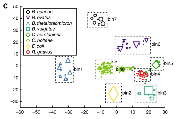
The approach of the authors was to first assemble the PacBio sequences, and then bin those larger genome fragments together based on a common epigenetic signature. 

Figure 2c shows the binning of genome fragments in a sample containing a known mixture of bacteria.

Figure 2e shows the binning of genome fragments in a gut microbiome sample containing a mixture of unknown bacteria (and viruses, fungi, etc.).

In general, this seems like a very interesting approach. After my read of the paper, it appears that the bacteria present in the microbiome contain a distinct enough set of epigenetic patterns to enable the deconvolution of many different species and strains. I look forward to seeing how this method stacks up against other binning approaches in the future. 

Final note

For those of you interested in phage and mobile genetic elements, I wanted to point out that the authors also explore a topic that has been studied somewhat by others – the linkage of phage to their hosts via epigenetic signatures. The idea here is that it can be computationally difficult to match a phage genome or plasmid with its host. One experimental method that accomplishes this is Hi-C, which takes advantage of the physical proximity of the host genome within an intact cell. In contrast, the PacBio method does not require intact cells, and can be used to link phage or plasmids with their host based on a shared epigenetic signature. 

My hope is that this type of data starts to become more widely available. There are clearly a number of computational tools that need to be refined in order to get full use of all this information, but it does seem to hold a good deal of promise. 

Making sparse DataFrames efficiently

Here's a little story about a computational challenge that I came across recently, and how a little bit of performance profiling went a long way to improve my analysis.

Background

I've been working with a large amount of data recently, and my principal bottleneck hasn't been the raw sequence analysis, but rather analyzing the results across large numbers of samples. For context, I'm working with thousands of samples, each of which contains 10,000 - 10,000,000 observations. The raw data was terabytes of raw genomic sequence data, and so I'm definitely working with a more compact data structure, but it's still quite a bit of data to work with in memory. 

There have been a few different iterations for this workflow, starting by working in memory (started swapping), then moving to a PostgreSQL database (which was too slow with read/write), and now working in memory on a larger machine using sparse matrices (following a helpful suggestion from Jonathan Golob).

What I've really liked about these sparse matrices is that it's incredibly fast to slice the data in different ways, which is what I need to be able to figure out both (a) how similar samples are to each other and (b) how different observations are distributed across samples. In other words, I need to be able to retrieve the data quickly in a column-wise or row-wise manner and sparse matrices really help with this.  Also, my underlying data is very sparse, which is to say that a vast majority of the cells in my table are 0 or N/A. Lastly, they're supported in Pandas, which is really great. 

The Challenge

While it's really quick to query these sparse matrices, I've been finding it difficult to make them. This morning I did a bit of performance profiling to compare a few different ways of constructing these tables and I found that not all construction methods are created equal. You can find my profiling code here, if you're interested (this was run in Pandas 0.20.3). 

The data that I'm working with is a set of observations that are originally constructed in longitudinal format, with every observation as an item in a list that includes the row name, column name, and cell value. What I wanted to see was what the most efficient method would be to make this into a sparse table in wide format, which could be indexed and sliced easily by row or column. 

Options

1. Sparse DataFrame from nested dictionaries: Make a nested dictionary with the first level of keys as column labels and the second level of keys as row labels, and then convert directly to the SparseDataFrame.

2. Column-wise addition to sparse DataFrame: Make an empty SparseDataFrame and then sequentially add in the data from each column. 

3. Dense longitudinal, pivot, then make sparse: Make a dense DataFrame from the longitudinal data, pivot it in dense format, and then make it into a SparseDataFrame.

4. Sparse longitudinal DataFrame, then pivot: Make a SparseDataFrame in longitudinal format and then pivot it in to wide format. 

Results

I tested each of the above options using four different matrices of varying sizes:

Matrix: 60 rows, 67 cols, 2.463% full

1. Testing sparse DataFrame from nested dictionaries
29.6 ms ± 2.33 ms per loop (mean ± std. dev. of 7 runs, 10 loops each)

2. Testing columnwise addition to sparse DataFrame
41.5 ms ± 813 µs per loop (mean ± std. dev. of 7 runs, 10 loops each)

3. Testing make dense DataFrame from longitudinal format, pivot it, then convert to sparse
33.1 ms ± 1.07 ms per loop (mean ± std. dev. of 7 runs, 10 loops each)

4. Testing make sparse DataFrame from longitudinal format, then pivot it
19 ms ± 1.39 ms per loop (mean ± std. dev. of 7 runs, 100 loops each)


Matrix: 100 rows, 100 cols, 9.54% full

1. Testing sparse DataFrame from nested dictionaries
61.2 ms ± 8.28 ms per loop (mean ± std. dev. of 7 runs, 10 loops each)

2. Testing columnwise addition to sparse DataFrame
97.7 ms ± 15 ms per loop (mean ± std. dev. of 7 runs, 10 loops each)

3. Testing make dense DataFrame from longitudinal format, pivot it, then convert to sparse
57.3 ms ± 2.15 ms per loop (mean ± std. dev. of 7 runs, 10 loops each)

4. Testing make sparse DataFrame from longitudinal format, then pivot it
101 ms ± 4.46 ms per loop (mean ± std. dev. of 7 runs, 10 loops each)


Matrix: 100 rows, 632 cols, 1.574% full

1. Testing sparse DataFrame from nested dictionaries
1.29 s ± 50.7 ms per loop (mean ± std. dev. of 7 runs, 1 loop each)

2. Testing columnwise addition to sparse DataFrame
1.41 s ± 40.4 ms per loop (mean ± std. dev. of 7 runs, 1 loop each)

3. Testing make dense DataFrame from longitudinal format, pivot it, then convert to sparse
1.19 s ± 13.6 ms per loop (mean ± std. dev. of 7 runs, 1 loop each)

4. Testing make sparse DataFrame from longitudinal format, then pivot it
94 ms ± 1.07 ms per loop (mean ± std. dev. of 7 runs, 10 loops each)


Matrix: 100 rows, 1000 cols, 9.526% full

1. Testing sparse DataFrame from nested dictionaries
2.82 s ± 29.1 ms per loop (mean ± std. dev. of 7 runs, 1 loop each)

2. Testing columnwise addition to sparse DataFrame
3.15 s ± 81.9 ms per loop (mean ± std. dev. of 7 runs, 1 loop each)

3. Testing make dense DataFrame from longitudinal format, pivot it, then convert to sparse
2.8 s ± 72.5 ms per loop (mean ± std. dev. of 7 runs, 1 loop each)

4. Testing make sparse DataFrame from longitudinal format, then pivot it
826 ms ± 30.8 ms per loop (mean ± std. dev. of 7 runs, 1 loop each)

Summary

In the results above you can see that in general the fastest method was #4 – making the DataFrame sparse in longitudinal format, and then pivoting it into wide matrix format. However, I need to stress that the relative performance of each of these methods varied widely depending on how sparse the matrix was. In general, option #4 worked better with sparser datasets, but I haven't fully tested the range of parameter space varying the number of rows, columns, and values. 

A larger point that I could also make here is that picking the right data structure for your project is actually a pretty tricky problem. I found here that the advantages of sparse matrices was immense relative to relational databases, but that they come with an up-front cost of matrix construction. I'm a biologist, not a computational scientist, and so the only way that I find my way through is by talking to smart people and incorporating their suggestions wherever appropriate. If you come up against a similar problem dealing with largish data, just take a deep breath, ask for help, and then write some tests.